torch.log1p() Method in PyTorch

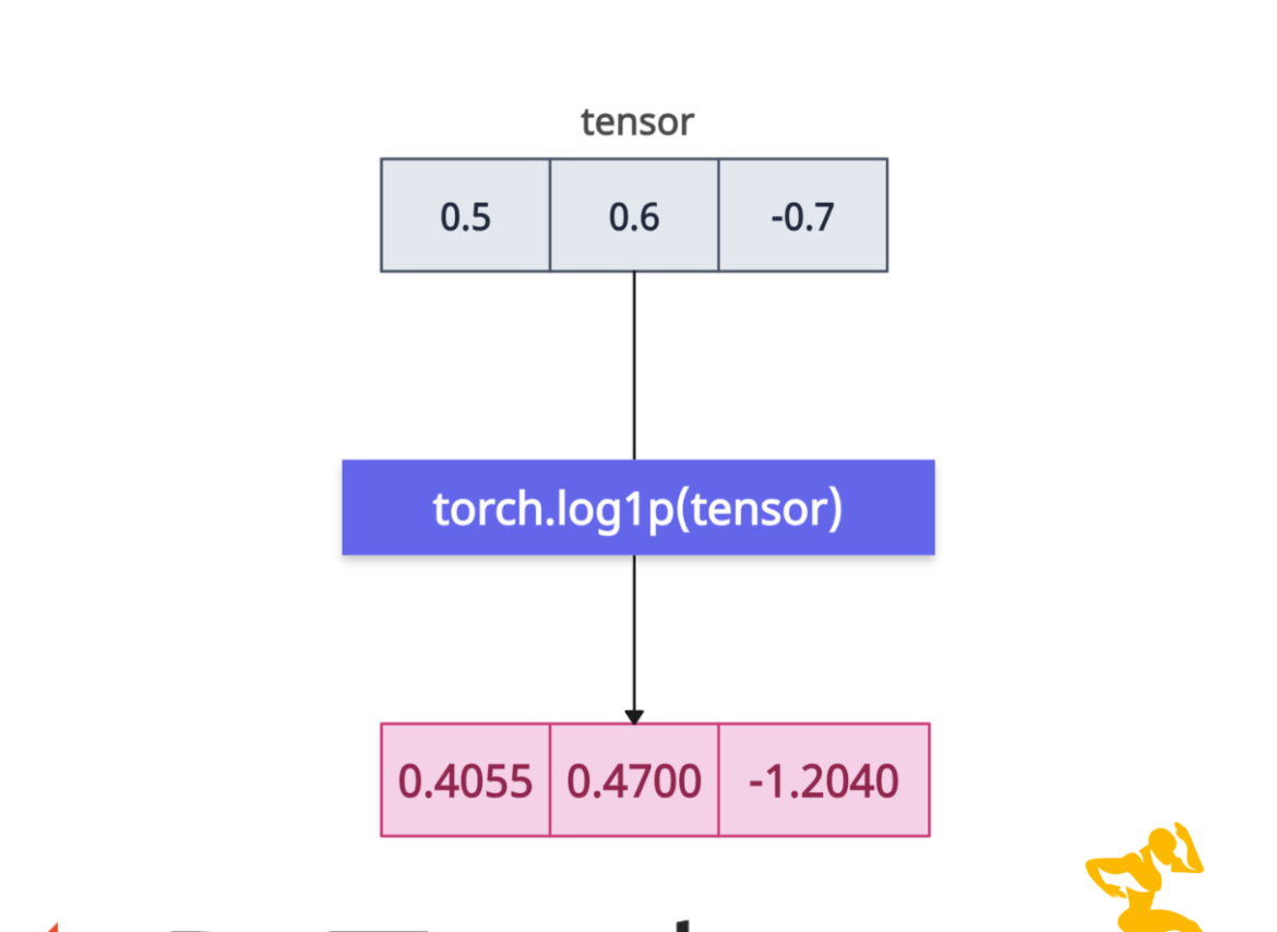
The torch.log1p() method calculates the natural logarithm of 1 + input element-wise.

For example, log1p() is more accurate than log(1 + x) because log1p() offers high precision, especially when x is close to zero. It provides improved numerical stability and calculates accurate results for small x where 1 + x is close to 1.

Syntax

torch.log1p(input, out=None)

Parameters

Name	Arguments
input (Tensor)	It represents an input tensor of any shape. It may contain non-negative values. Though negative values are valid where 1 + x > 0.
out (Tensor, optional)	By default, it is None, but if you have a pre-allocated tensor, you can use this argument to store the result.

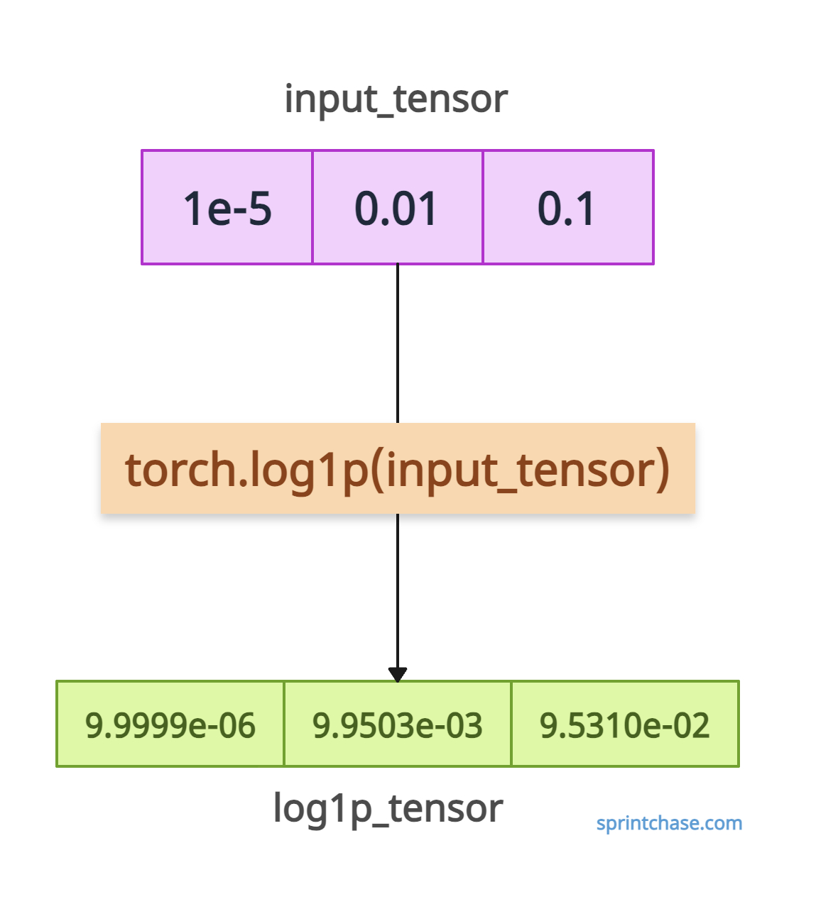
Calculating log1p() for small inputs

Let’s use log1p() and log(1 + x) to compare both results and see why log1p() is more accurate.

import torch

input_tensor = torch.tensor([1e-5, 0.01, 0.1])

log1p_tensor = torch.log1p(input_tensor)
print(log1p_tensor)
# Output: tensor([9.9999e-06, 9.9503e-03, 9.5310e-02])

# Compare with torch.log(1 + x)
unstable = torch.log(1 + input_tensor)
print(unstable)
# Output: tensor([1.0014e-05, 9.9503e-03, 9.5310e-02])

In the above code, you can see that for input_tensor element = 1e-5, log1p ensures accuracy, while log(1 + x) may suffer from precision loss in extreme cases (e.g., x < 1e-8).

Negative values

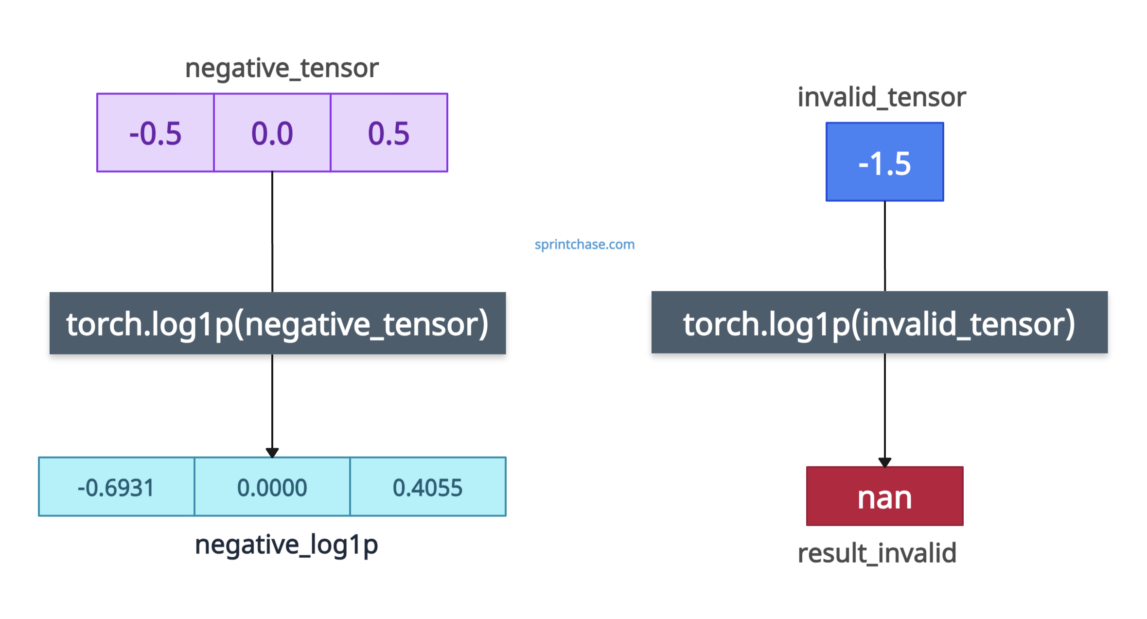
It will allow negative values as long as 1 + input > 0, which means the input value should be greater than -1 (input > -1). If the input is ≤ −1, it will yield -inf or nan.

import torch

negative_tensor = torch.tensor([-0.5, 0.0, 0.5])
negative_log1p = torch.log1p(negative_tensor)

print(negative_log1p)
# Output: tensor([-0.6931,  0.0000,  0.4055])

# Invalid input
invalid_tensor = torch.tensor([-1.5])

result_invalid = torch.log1p(invalid_tensor)

print(result_invalid)
# Output: tensor([nan])

You can see that as long as the input is greater than -1, it will return a valid tensor. Once your input is less than -1, it will return NaN.

Multi-dimensional tensors

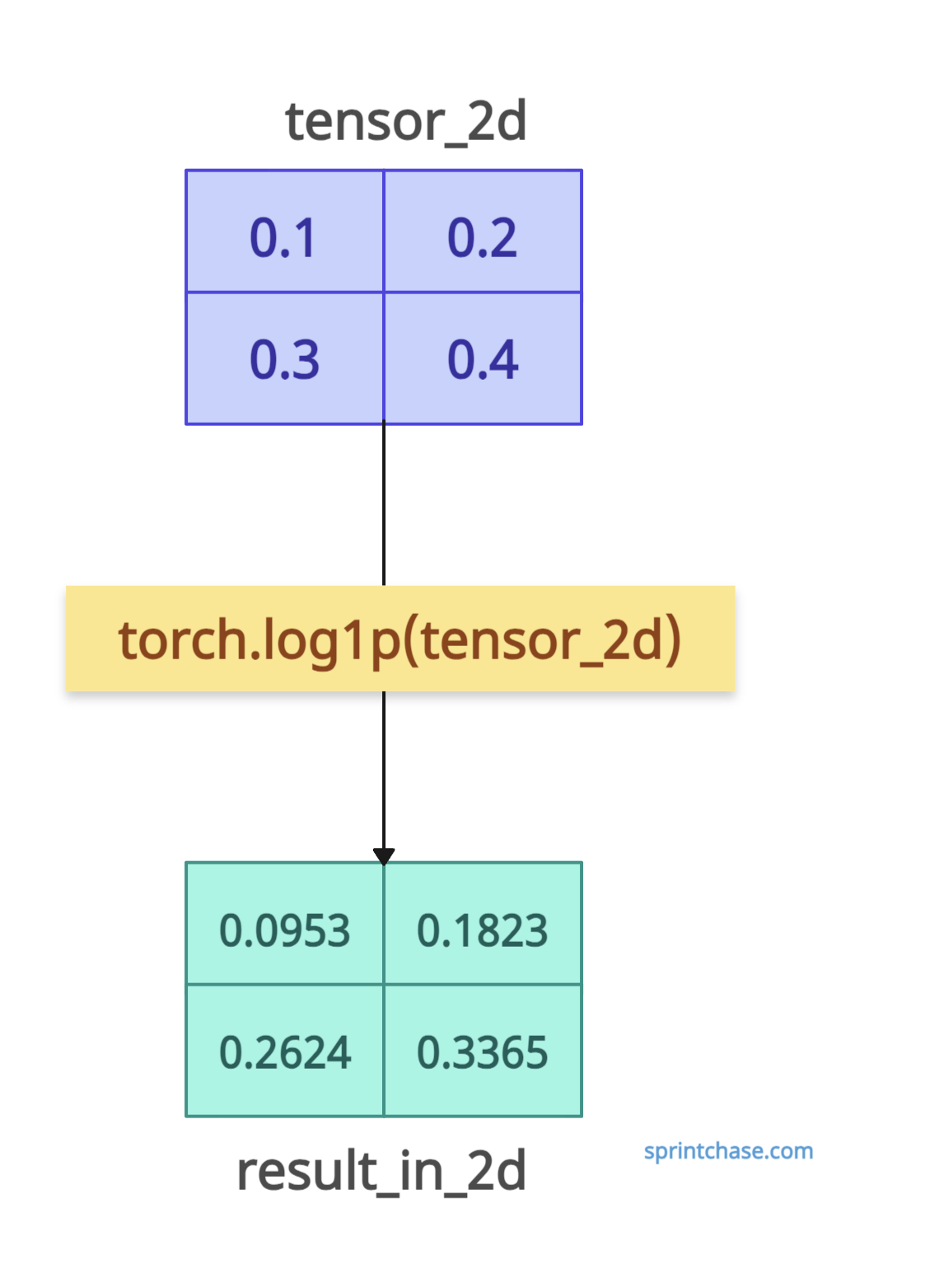
What if our input tensor is multi-dimensional? Well, it will calculate log1p() of a 2D tensor efficiently. If the input is 2D, the output will also be 2D.

import torch

tensor_2d = torch.tensor([[0.1, 0.2], [0.3, 0.4]])

result_in_2d = torch.log1p(tensor_2d)

print(result_in_2d)
# Output: tensor([[0.0953, 0.1823],
#                 [0.2624, 0.3365]])

From the output, we can see that log1p applies element-wise, preserving the input tensor’s shape.

Plotting

Let’s visualize the log1p() values on the chart using the matplotlib library. If you have not installed it, you can install it using the pip install matplotlib command.

import torch
import matplotlib.pyplot as plt

# Generate input values
x = torch.linspace(-0.9, 1.0, 100)

# Compute log1p
log1p_y = torch.log1p(x)

# Convert to numpy for plotting
x_np = x.numpy()
log1p_y_np = log1p_y.numpy()

# Create the plot
plt.figure(figsize=(8, 6))
plt.plot(x_np, log1p_y_np, label='torch.log1p(x)',
         color='#1f77b4', linewidth=2)
plt.xlabel('x')
plt.ylabel('Output')
plt.title('torch.log1p(x)')
plt.grid(True)
plt.legend()
plt.show()

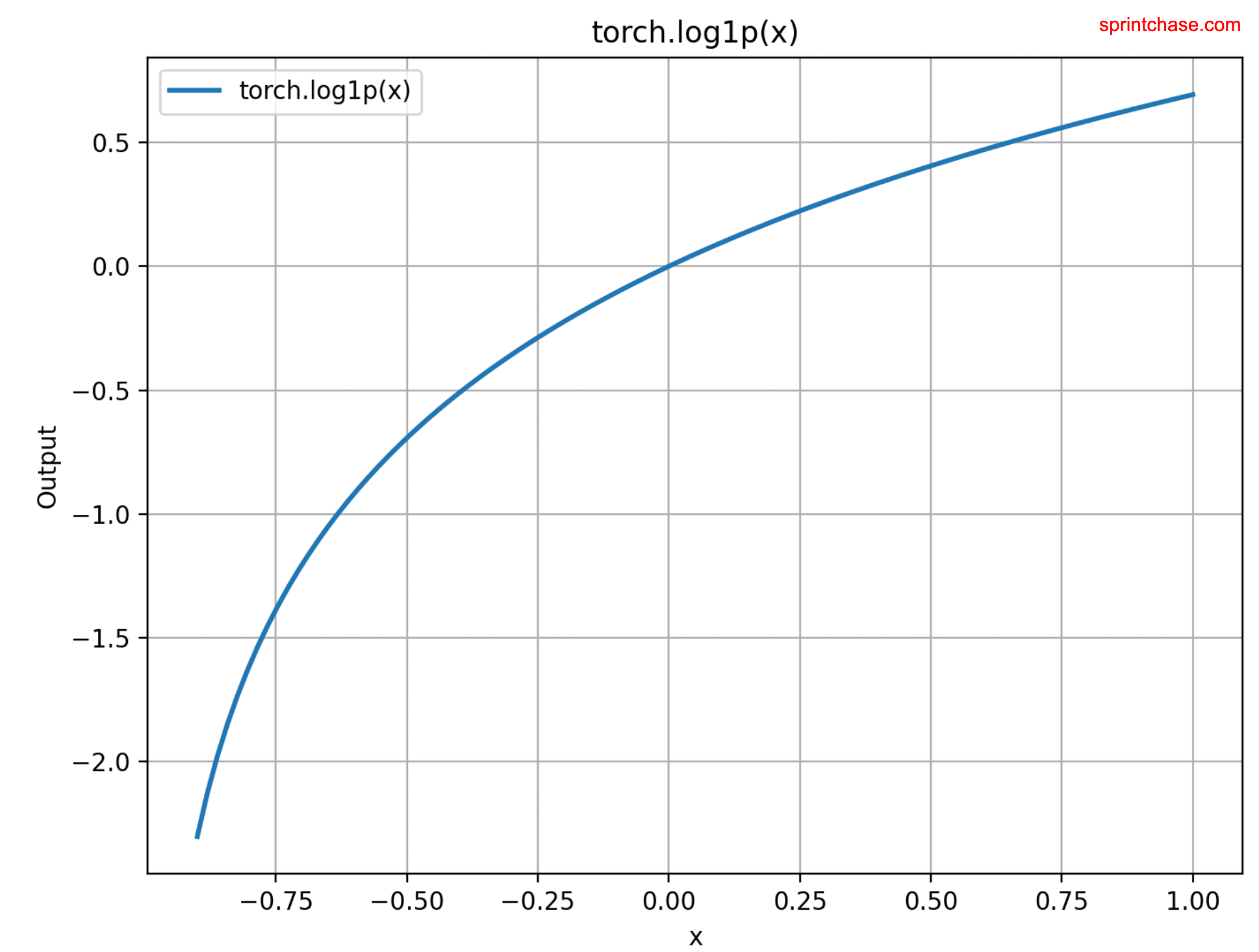
In the above code, we generated input values using torch.linspace() method. To plot these values, we need to convert them into a numpy array using the .numpy() method.

Then, using matplotlib’s methods, we plotted a chart.